Ensemble/Boosting

Ensemble Methods

• use an ensemble/group of hypotheses
• diversity important; ensemble of “yes-men” is useless

• get diverse hypotheses by using

  • different data
  • different algorithms
  • different hyperparameters

Why?

• averaging reduces variance

  • ensemble more stables than individual

  • consider biased coin p(head) = 1/3

    • variance on one flip = 1/3 - 1/9 = 2/9
    • variance on average of 2 flips = 2/9 - 1/9 = 1/9

• averaging makes less mistakes

  • consider 3 classifiers with accuracy 0.8, 0.7, and 0.7
  • the probability that the majority vote is correct = (f1 correct, f2 correct, f3 wrong) + (f1 correct, f2 wrong, f3 correct) + (f1 wrong, f2 correct, f3 correct) + (f1 correct, f2 correct, f3 correct)
  • = \((.8*.7*.3) + (.8*.3*.3) + (.2*.7*.7) + (.8*.8*.7) \approx 0.82\)

Creation

• use different training sets

  • bootstrap example: pick m examples from labeled data with replacement
  • cross-validation sampling
  • reweight data (boosting, later)

• use different features

  • random forests “hide” some features

Prediction

• unweighted vote

• weighted vote

  • pay more attention to better predictors

• cascade

  • filter examples; each level predicts or passes on

Boosting

• “boosts” the preformance of another learning algorithm
• creates a set of classifiers and predicts with weighted vote

• use different distributions on sample to get diversity

  • up-weight hard, down-weight easy examples

• note: ensembles used before to reduce variance

If boosting is possible, then:

• can use fairly wild guesses to produce highly accurate predictions
• if you can learn “part way” you can learn “all the way”
• should be able to improve any learning algorithm

• for any learning problem:

  • either can learn always with nearly perfect accuracy
  • or there exist cases where cannot learn even slightly better than random guessing

Ada-Boost

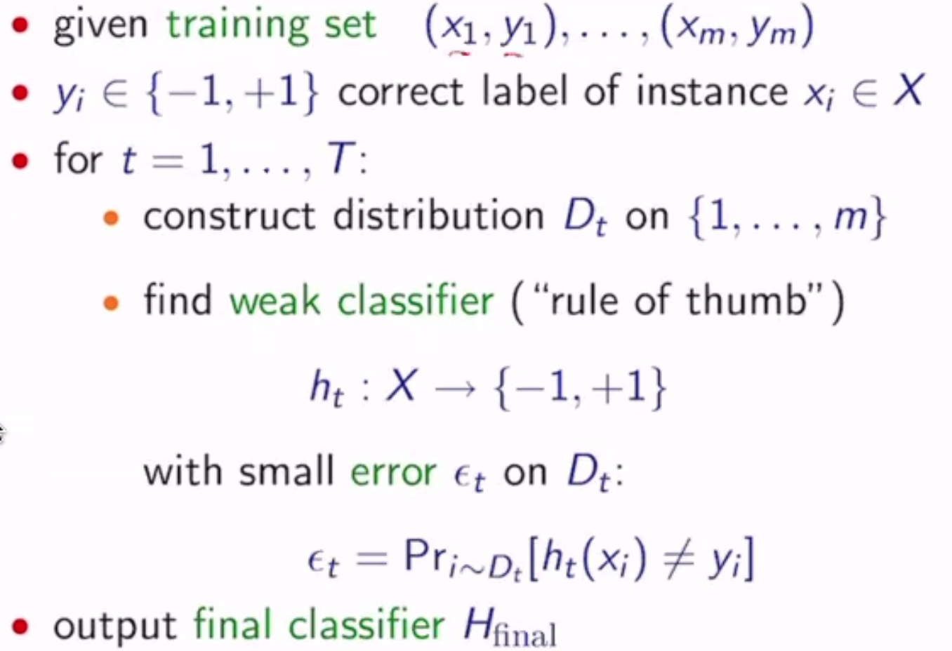
Given a training sample S with labels +/-, and a learning algorithm L:

1. for t from 1 to T do

   1. create distribution \(D_t\) on \(S\)

   2. call \(L\) with \(D_t\) on \(S\) to get hypothesis \(h_t\)

      1. i.e. \(\min \sum_n D_t(n) l(f(x_n), y_n)\) where \(D_t(n)\) is the weight of the sample

   3. calculate weight \(\alpha_t\) for \(h_t\)

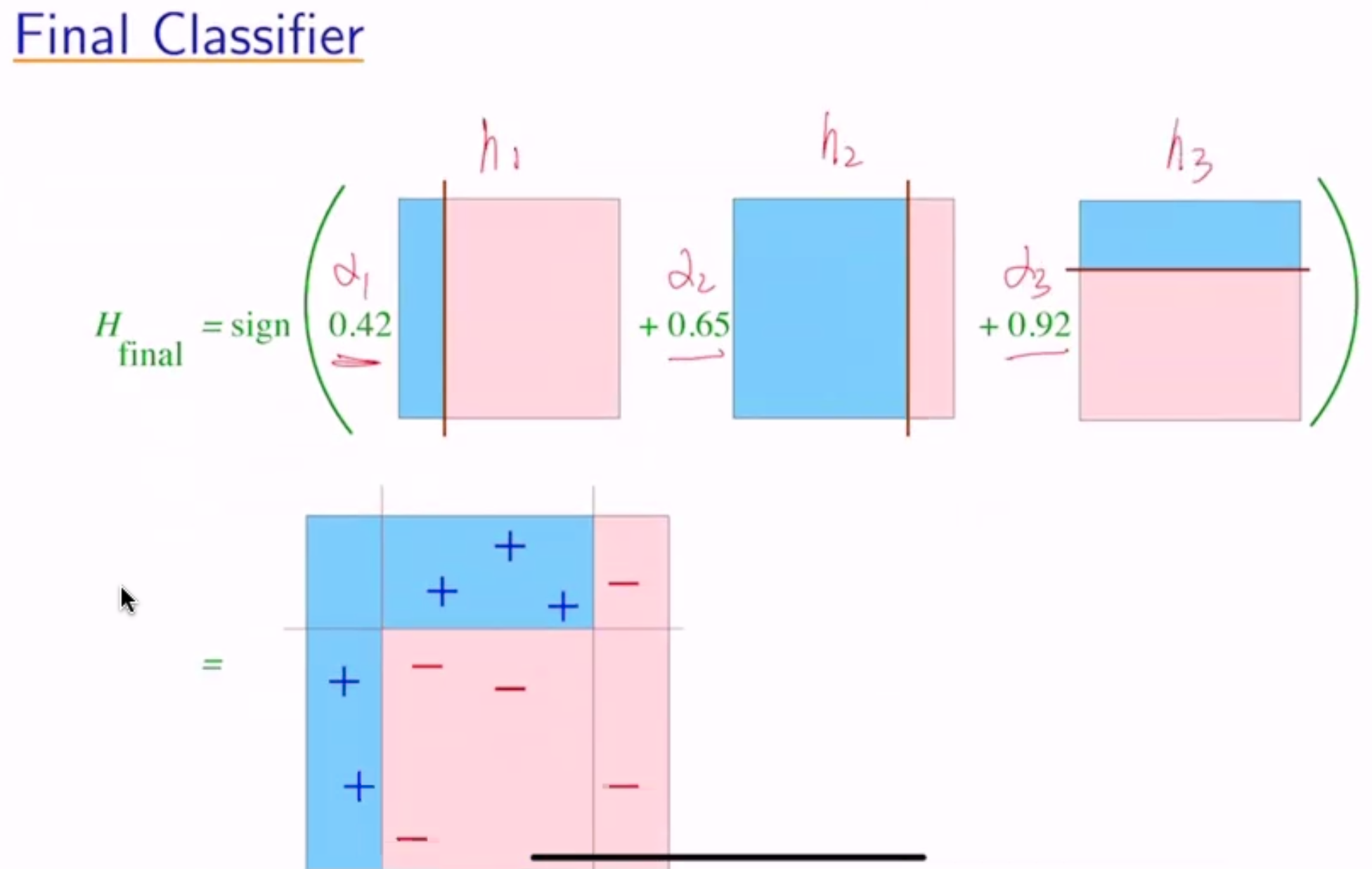
2. final hypothesis is \(F(x) = \sum_t \alpha_t h_t(x)\), or \(H(x)\) = value with most weight

formally:

So how do we pick \(D_t\) and \(\alpha_t\)?

• \(D_1(i) = 1/m\) - the weight assigned to \((x_i, y_i)\) at \(t=1\)

• given \(D_t\) and \(h_t\):

  • \(D_{t+1}(i) = \frac{D_t(i)}{Z_t} \exp(-\alpha_t y_i h_t(x_i))\)

    • if correct, increase weights by a factor > 1 (positive exponential)
    • otherwise decrease by a factor < 1 (negative exponential)

  • where \(Z_t\) is a normalization factor
  • where \(\alpha_t = \frac{1}{2} \ln (\frac{1-\epsilon_t}{\epsilon_t}) > 0\)

• \(H_{final}(x) = sign(\sum_t \alpha_t h_t(x))\)

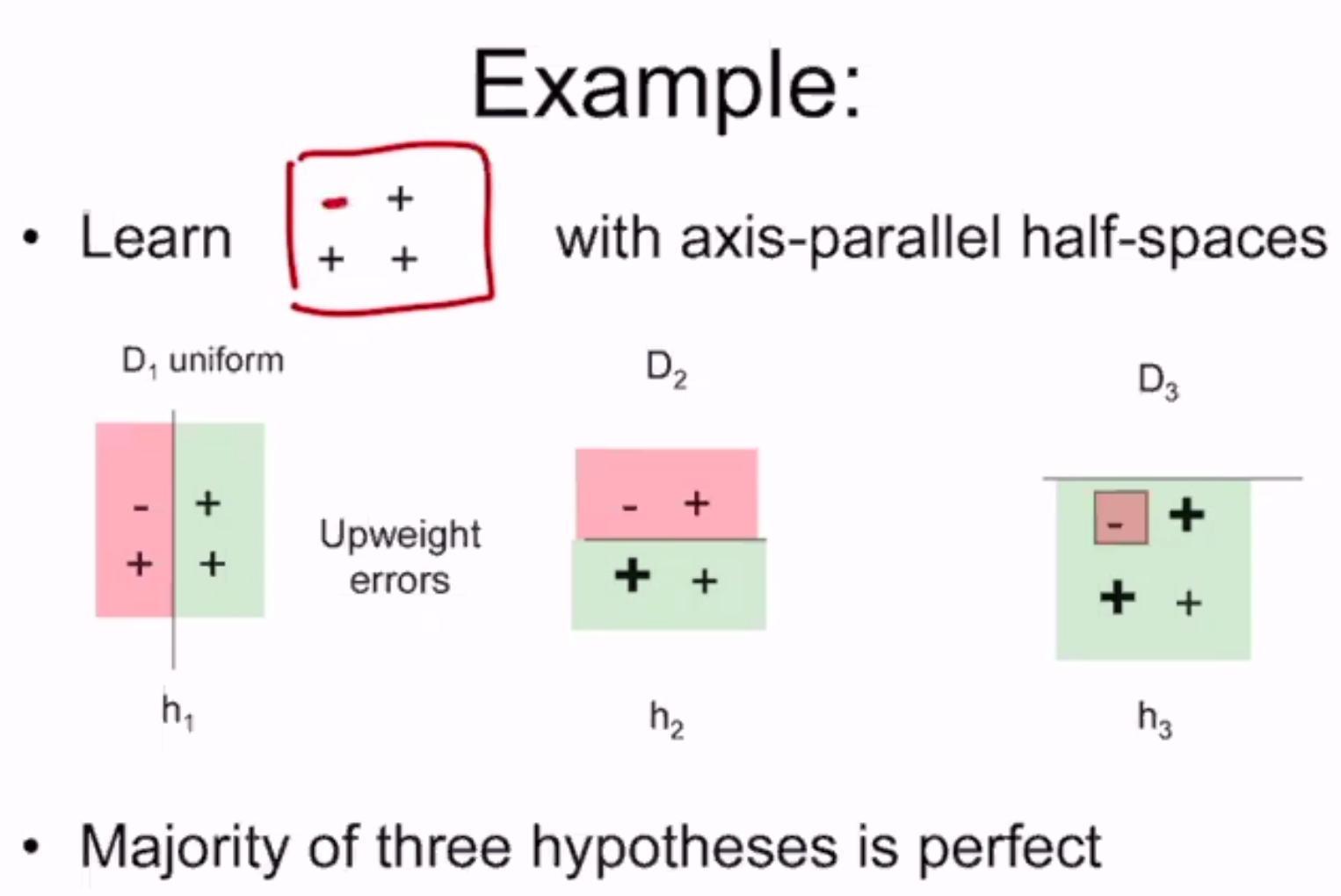
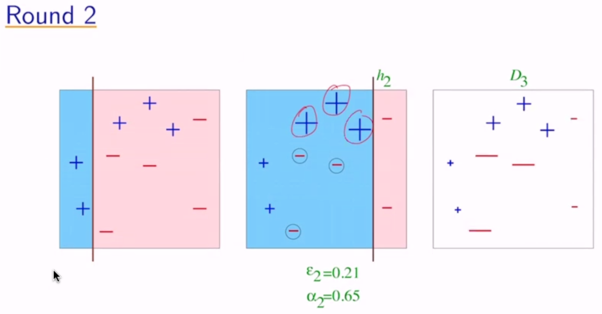
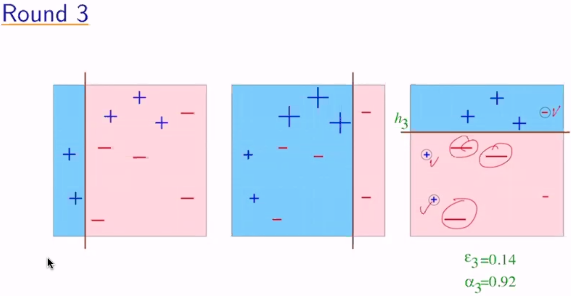
Example:

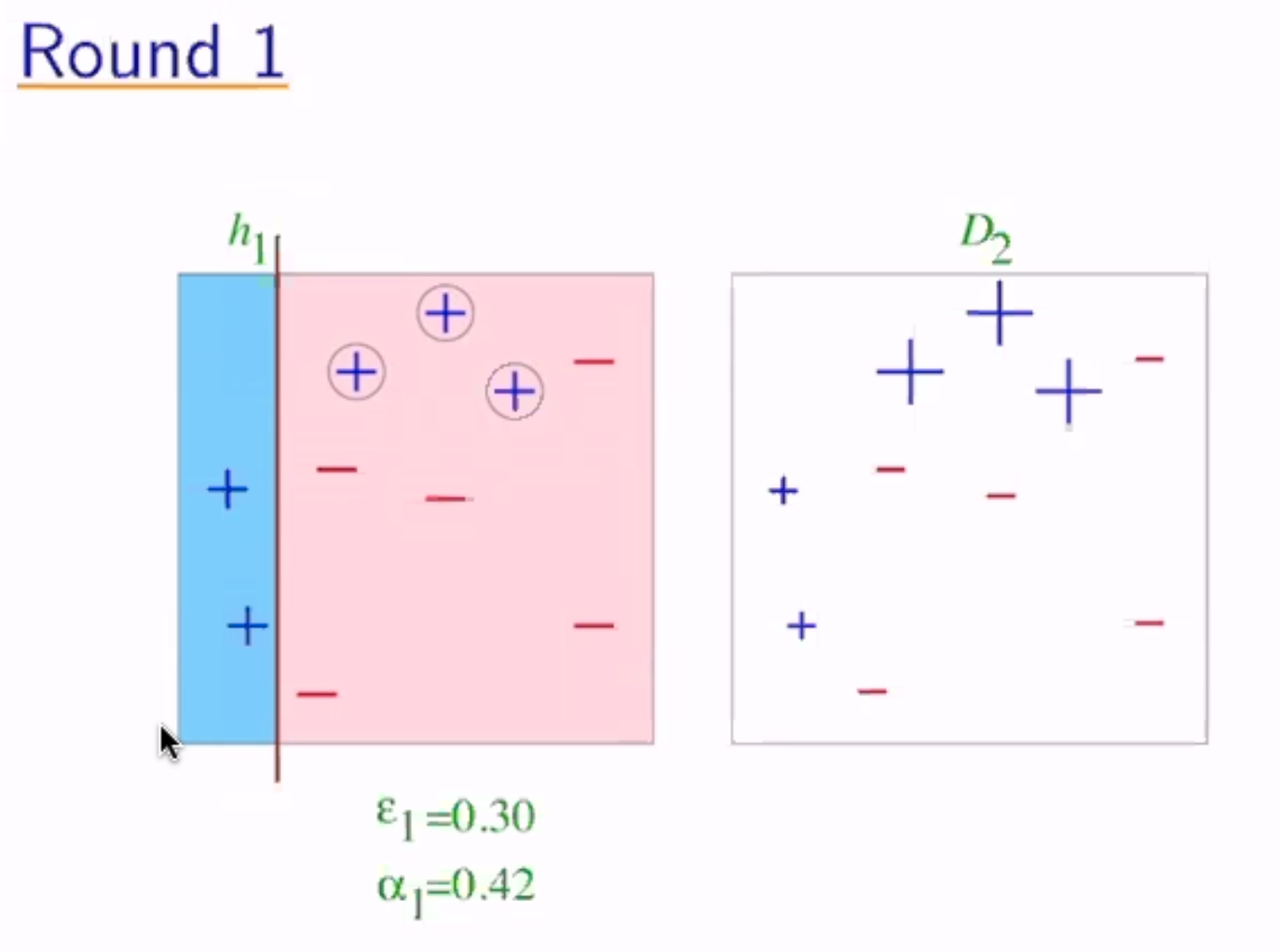
now the weights become \(\frac{1}{10} e^{0.42}\) for the misclassified and \(\frac{1}{10} e^{-0.42}\) for the correct

Analyzing Error

Thm: Write \(\epsilon_t\) as \(1/2 - \gamma_t\) - \(\gamma_t\) = “edge” = how much better than random guessing. Then:

\[\begin{split}\text{training error}(H_{final}) & \leq \prod_t [2 \sqrt{\epsilon_t (1-\epsilon_t)}] \\ & = \prod_t \sqrt{1-4\gamma_t^2} \\ & \leq \exp(-2\sum_t \gamma_t^2)\end{split}\]

So if \(\forall t: \gamma_t \geq \gamma > 0\), then \(\text{training error}(H_{final}) \leq e^{-2\gamma^2 T}\)

therefore, as \(T \to \infty\), training error \(\to 0\)

Proof

Let \(F(x) = \sum_t \alpha_t h_t(x) \to H_{final}(x) = sign(F(x))\)

Step 1: unwrapping recurrence

\[\begin{split}D_{final}(i) & = \frac{1}{m} \frac{\exp(-y_i \sum_t \alpha_t h_t(x_i))}{\prod_t Z_t} \\ & = \frac{1}{m} \frac{\exp(-y_i F(x_i))}{\prod_t Z_t}\end{split}\]

Step 2: training error \((H_{final}) \leq \prod_t Z_t\)

\[\begin{split}\text{training error}(H_{final}) & = \frac{1}{m} \sum_i & 1 & \text{ if } y_i \neq H_{final}(x_i) \\ & & 0 & \text{ otherwise} \\ & = \frac{1}{m} \sum_i & 1 & \text{ if } y_i F(x_i) \leq 0 \\ & & 0 & \text{ otherwise} \\ & \leq \frac{1}{m} \sum_t \exp(-y_i F(x_i)) \\ & = \sum_i D_{final}(i) \prod_t Z_t \\ & = \prod_t Z_t\end{split}\]

Step 3: \(Z_t = 2 \sqrt{\epsilon_t (1-\epsilon_t)}\)

\[\begin{split}Z_t & = \sum_i D_t(i) \exp(-\alpha_t y_i h_t(x_i)) \\ & = \sum_{i:y_i \neq h_t(x_i)} D_t(i)e^{\alpha_t} + \sum_{i:y_i = h_t(x_i)} D_t(i) e^{-\alpha_t} \\ & = \epsilon_t e^{\alpha_t} + (1-\epsilon_t) e^{\alpha_t} \\ & = 2 \sqrt{\epsilon_t (1-\epsilon_t)}\end{split}\]

Discussion

We expect even as training error approaches 0 as T increases, the test error won’t - overfitting!

We can actually predict “generalization error” (basically test error):

\[\text{generalization error} \leq \text{training error} + \tilde{O}(\sqrt{\frac{dT}{m}})\]

Where \(m\) = # of training samples, \(d\) = “complexity” of weak classifiers, \(T\) = # of rounds

But in reality, it’s not always a tradeoff between training error and test error.

Margin Approach

• training error only measures whether classifications are right or wrong
• should also consider confidence of classifications
• \(H_{final}\) is weighted majority vote of weak classifiers

• measure confidence by margin = strength of the vote

  • = (weighted fraction voting correctly) - (weighted fraction voting incorrectly)

• so as we train more, we increase the margin, which leads to a decrease in test loss

• both AdaBoost and SVMs

  • work by maximizing margins
  • find linear threshold function in high-dimensional space

• but they use different norms

AdaBoost is:

• fast
• simple, easy to program
• no hyperparameters (except T)
• flexible, can combine with any learning algorithm
• no prior knowledge needed about weak learner
• provably effective (provided a rough rule of thumb)
• versatile

But:

• performance depends on data and weak learner

• consistent with theory, adaboost can fail if:

  • weak classifiers too complex (overfitting)

  • weak classifiers too weak (basically random guessing)

    • underfitting, or low margins -> overfitting

• susceptible to uniform noise