SVMs

Note

On the homework:

\[\begin{split}& P(GPA=x|type=N) \\ & = \frac{1}{\sqrt{2\pi \sigma_N^2}} \exp(\frac{-(x-\mu_N)^2}{2\sigma_N^2})\end{split}\]

How do we estimate \(\mu\) and \(\sigma\) from the data?

1. \(\arg \max_{\mu, \sigma} P(GPA1, GPA2..GPA6|\mu, \sigma)\)
2. \(\hat{\mu}_N = avg(GPA)\)

Support Vector Machines

Max-Margin Classification

This is a linearly separable dataset, and all these hyperplanes are valid, but which one is best?

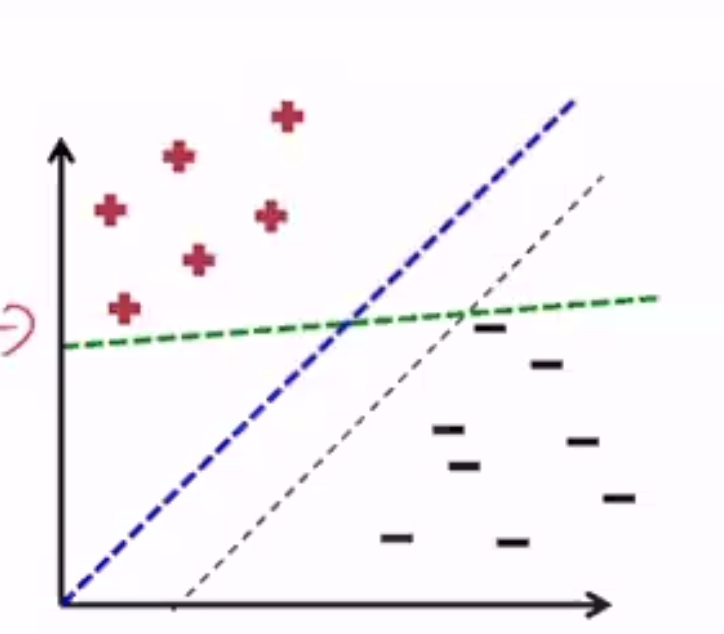
• The blue one has the largest margin

• Margin: Distance between the hyperplane and the nearest point

  • defined for a given dataset \(\mathbf{D}\) and hyperplane \((\mathbf{w}, b)\)

\[\begin{split}margin(\mathbf{D}, \mathbf{w}, b) = & \min_{(x, y)\in \mathbf{D}} y(\mathbf{w \cdot x} + b) & \text{ if w separates D} \\ & -\inf & \text{ otherwise}\end{split}\]

SVM is a classification algorithm that tries to find the maximum margin separating hyperplane.

Hard SVM

Setup

• Input: training set of pairs \(<x_n, y_n>\)

  • \(x_n\) is the D-dimensional feature vector
  • \(y_n\) is the label - assume binary \(\{+1, -1\}\)

• Hypothesis class: set of all hyperplanes H

• Output: \(w\) and \(b\) of the maximum hypotheses \(h\in H\)

  • \(w\) is a D-dimensional vector (1 for each feature)
  • \(b\) is a scalar

Prediction

• learned boundary is the maximum-margin hyperplane specified by \(w, b\)
• given a test instance \(x'\), prediction \(\hat{y} = sign(w \cdot x' + b)\)
• if the prediction is correct, \(\hat{y}(w \cdot x' + b) > 0\)

Intuition

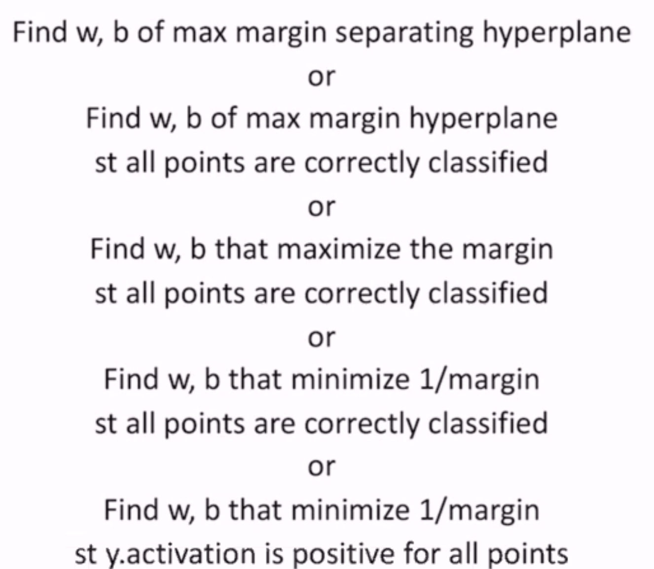
But \(y * activation\) is a weak condition - let’s increase it to be “sufficiently” positive

Final Goal: Find w, b that minimize 1/margin s.t. y * activation >= 1 for all points

Optimization

\[\begin{split}\min_{w, b} & \frac{1}{\gamma(w, b)} \\ \text{subj. to } & y_n(w \cdot x_n + b) \geq 1 (\forall n)\end{split}\]

Where \(\gamma\) is the distance from the hyperplane to the nearest point

• maximizing \(\gamma\) = minimizing \(1/\gamma\)

• constraints: all training instances are correctly classified

  • we have a 1 instead of 0 in the condition to ensure a non-trivial margin
  • this is a hard constraint, and so called a hard-margin SVM

• what about for non linearly-separable data?

  • infeasible solution (feasible set is empty): no hyperplane tielded
  • let’s loosen the constraint slightly

Soft-Margin SVMs

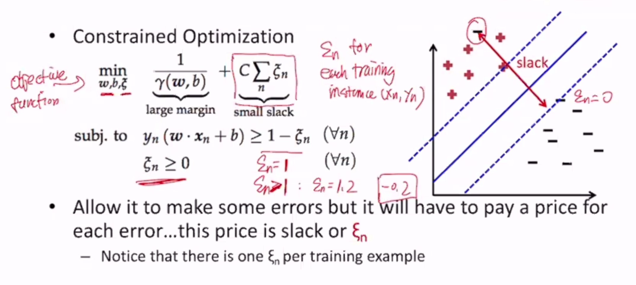
• introduce one slack variable \(\xi_n\) for each training instance

• if a training instance is classified correctly, \(\xi_n\) is 0 since it needs no slack

  • but \(\xi_n\) can even be >1 for incorrectly classified instances
  • if \(\xi_n\) is 0, classification is correct
  • if \(0 < \xi_n < 1\), classification is correct but margin is not large enough
  • if \(\xi_n > 1\), classification is incorrect

• where \(C\) is a hyperparameter (how much to care about slack)

  • if the slack component of the objective function is 0, it’s the same goal as a hard-margin SVM

TLDR: maximize margin while minimizing total cost the model has to pay for misclassification that happens while obtaining this margin

Discussion

Note that the max-margin hyperplane lies in the middle between the positive and negative points

• So the margin is determined by only 2 data points, that lie on the lines \(w \cdot x + b = 1\) and \(w \cdot x + b = -1\)
• these points, \(x_+\) and \(x_-\), are called support vectors

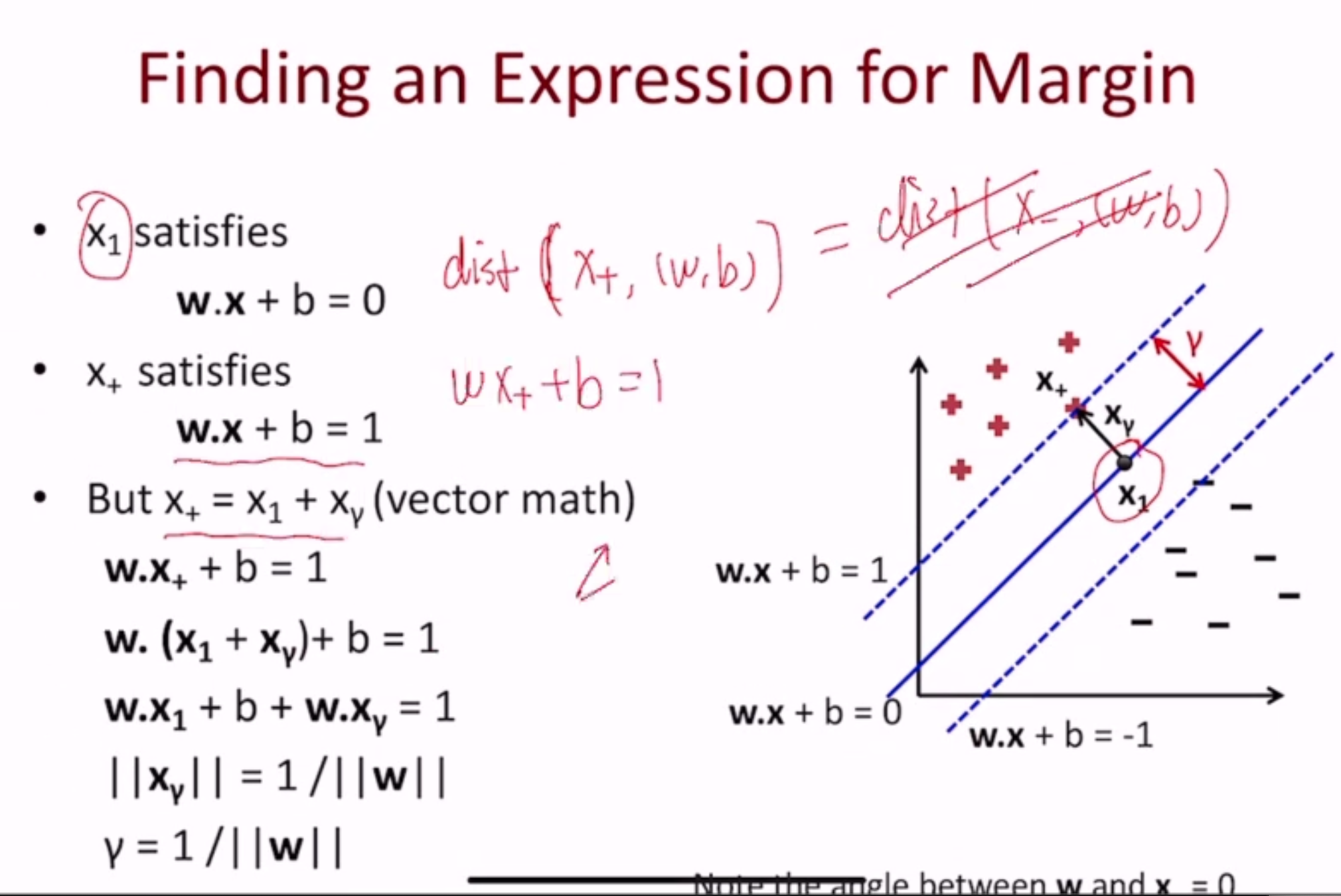
Note

\(w \cdot x_1 + b\) is 0 since \(x_1\) is on the decision boundary

\(w \cdot x_\gamma = 1\) -> \(||w||*||x_\gamma|| = 1\) since \(w, x_\gamma\) are parallel

Therefore, we can modify the objective:

\[\begin{split}\min_{w, b, \xi} & \frac{1}{2}||w||^2 + C\sum_n \xi_n & \\ \text{subj. to } & y_n(w \cdot x_n + b) \geq 1 - \xi_n & (\forall n) \\ & \xi_n \geq 0 & (\forall n)\end{split}\]

Or, intuitively, finding the smallest weights possible.

Hinge Loss

We can write the slack variables in terms of \((w, b)\):

\[\begin{split}\xi_n = & 0 & \text{ if } y_n(w\cdot x_n + b) \geq 1 \\ & 1 - y_n(w\cdot x_n + b) & \text{ otherwise}\end{split}\]

which is hinge loss! Now, the SVM objective becomes:

\[\min_{w, b} \frac{1}{2}||w||^2 + C\sum_n l^{(hin)}(y_n, w\cdot x_n + b)\]

Solving

Hard-Margin SVM

\[\begin{split}\min_{w, b} & \frac{1}{2}||w||^2 \\ \text{subj. to } & y_n(w \cdot x_n + b) \geq 1 (\forall n)\end{split}\]

• convex optimization problem

• specifically a quadratic programming problem

  • minimizing a function that is quadratic in vars
  • constraints are linear

• this is called the primal form, but most people solve the dual form

We can encode the primal form algebraically:

\[\min_{w, b} \max_{\alpha \geq 0} \frac{1}{2}(w \cdot w) + \sum_i \alpha_i (1-y_i(w \cdot x_i + b))\]

Dual Form

• does not change the solution
• introduces new variables \(\alpha_n\) for each training instance

\[\begin{split}\max & \sum_{n=1}^N \alpha_n - \frac{1}{2} \sum_{m,n=1}^N \alpha_m \alpha_n y_m y_n (x_m^T x_n) \\ \text{subject to } & \sum_{n=1}^N \alpha_n y_n = 0, \alpha_n \geq 0; n = 1..N\end{split}\]

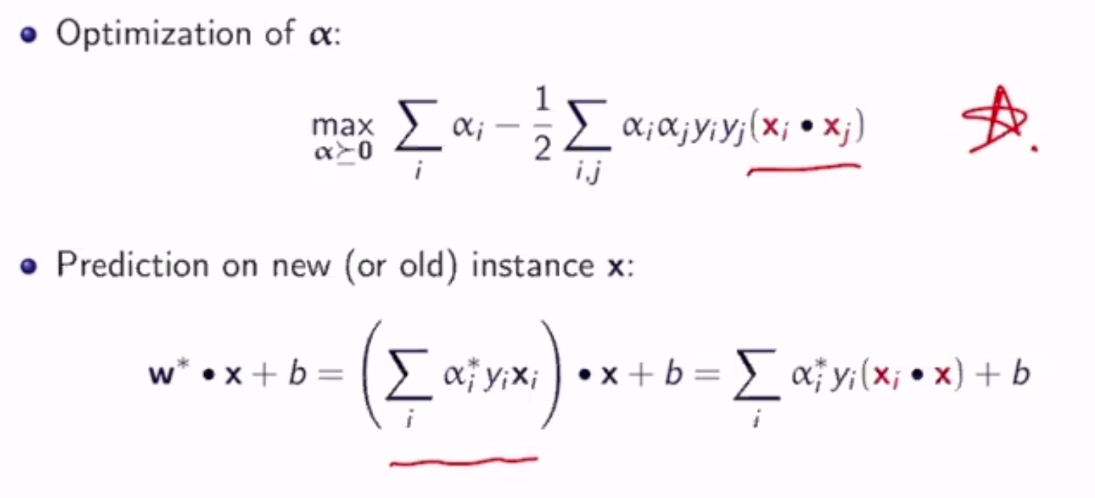
Once the \(\alpha_n\) are computed, w and b can be computed as:

\[\begin{split}w = \sum_{n=1}^N \alpha_n y_n x_n \\ b = \text{something...}\end{split}\]

As it turns out, most \(\alpha_i\)’s are 0 - only the support vectors are not

For Soft-Margin SVM

\[\begin{split}\max & \sum_{n=1}^N \alpha_n - \frac{1}{2} \sum_{m,n=1}^N \alpha_m \alpha_n y_m y_n (x_m^T x_n) \\ \text{subject to } & \sum_{n=1}^N \alpha_n y_n = 0, 0 \leq \alpha_n \leq C; n = 1..N\end{split}\]

For soft-margin SVMs, support vectors are:

• points on the margin boundaries (\(\xi = 0\))
• points in the margin region (\(0 < \xi < 1\))
• points on the wrong side of the hyperplane (\(\xi \geq 1\))

Conclusion: w and b only depend on the support vectors

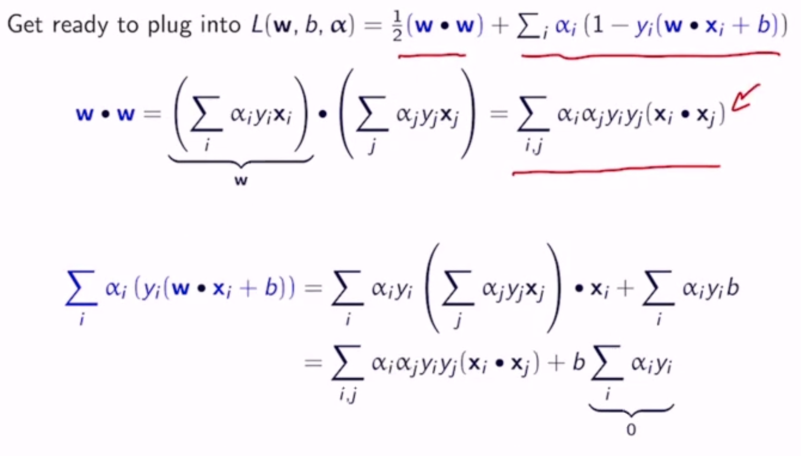
Derivation

Given the algebriaecally encoded primal form:

\[\min_{w, b} \max_{\alpha \geq 0} \frac{1}{2}(w \cdot w) + \sum_i \alpha_i (1-y_i(w \cdot x_i + b))\]

We can switch the order of the min and max:

\[\begin{split}\max_{\alpha \geq 0} \min_{w, b} \frac{1}{2}(w \cdot w) + \sum_i \alpha_i (1-y_i(w \cdot x_i + b)) \\ = \max_{\alpha \geq 0} \min_{w, b} L(w, b, \alpha)\end{split}\]

To solve inner min, differentiate L wrt w and b:

\[\begin{split}\frac{\partial L(w, b, \alpha)}{\partial w_k} & = w_k - \sum_i \alpha_i y_i x_{i,k} & \\ \frac{\partial L(w, b, \alpha)}{\partial w} & = w - \sum_i \alpha_i y_i x_i & \to w = \sum_i \alpha_i y_i x_i \\ \frac{\partial L(w, b, \alpha)}{\partial b} & = - \sum_i \alpha_i y_i & \to \sum_i \alpha_i y_i = 0\end{split}\]

• \(w = \sum_i \alpha_i y_i x_i\) means w is a weighted sum of examples
• \(\sum_i \alpha_i y_i = 0\) means positive and negative examples have the same weight
• \(\alpha_i > 0\) only when \(x_i\) is a support vector, so w is a sum of signed support vectors

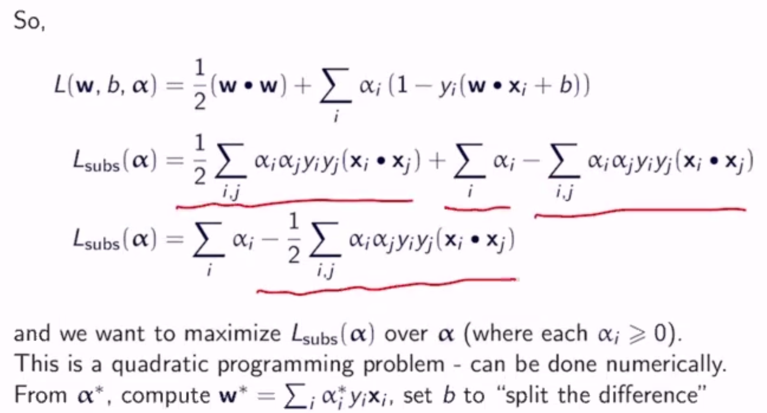
Conclusion

Soft-Margin

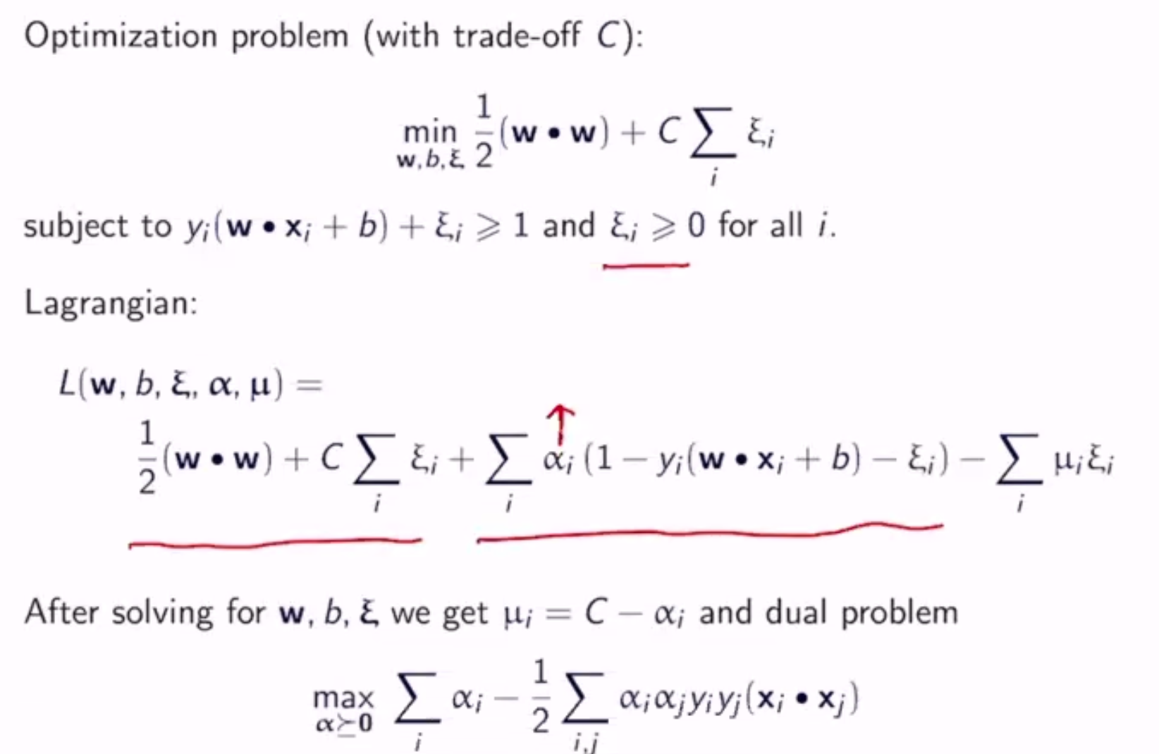
subject to \(0 \leq \alpha_i \leq c\) \((\forall i)\)

Non-Linearly-Seperable

What if our data is not linearly seperable?

• use a non-linear classifier

• transform our data so that it is, somehow

  • e.g. adding a dummy dimension based on a quadratic formula of the real dimension

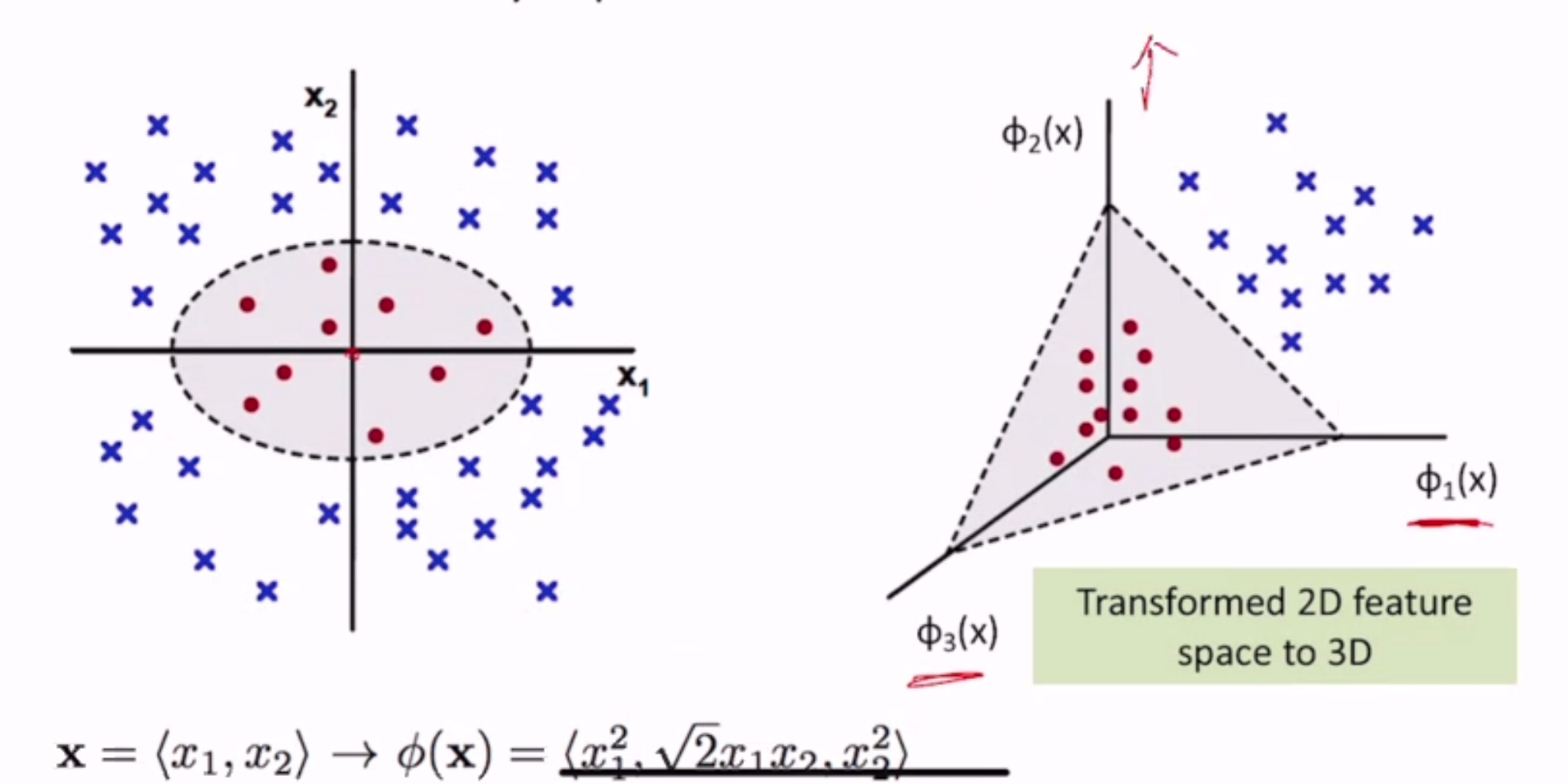
Feature Mapping

We can map the original feature vector to a higher dimensional space \(\phi(x)\)

e.g. quadratic feature mapping:

\[\begin{split}\phi(x) = < & 1, 2x_1, 2x_2, ..., 2x_D, \\ & x_1^2, x_1x_2, ..., x_1x_D, \\ & x_2x_1, x_2^2, ..., x_2x_D, \\ & ... >\end{split}\]

Pros: this improves separability, you can apply a linear model more confidently

Cons: There are a lot more features now, and a lot of repeated features - lots of computation and easier to overfit