Kernel Methods

• step 1: use a special type of mapping functions

  • still map feature space to a higher dimensional space
  • but computation of \(\phi(x) \cdot \phi(z)\) is easy (remember the multiplication of features in SVM optimization)

• step 2: rewrite the model s.t.

  • the mapping \(\phi(x)\) never needs to be explicitly computed - i.e. never compute terms like \(w \cdot \phi(x) + b\)
  • only work with \(\phi(x) \cdot \phi(z)\) - we call this the kernel function

Ex.

\[\mathbf{x} = <x_1, x_2> \to \phi(x) = <x_1^2, \sqrt{2}x_1 x_2, x_2^2>\]

We can compute \(\phi(x) \cdot \phi(z)\) easily:

\[\begin{split}\phi(x) \cdot \phi(z) & = <x_1^2, \sqrt{2}x_1 x_2, x_2^2> \\ & = <x_1^2, \sqrt{2}x_1 x_2, x_2^2> \cdot <z_1^2, \sqrt{2}z_1 z_2, z_2^2> \\ & = ... \\ & = (x \cdot z)^2 \\ & = K(x, z)\end{split}\]

We call this a kernel function

What about the quadratic feature mapping?

\[... = (1+x \cdot z)^2 = K(x, z)\]

Kernel in SVM

Rewriting the primal form of the SVM to use the mapped space doesn’t seem easy.

But we can rewrite the dual form easily!

\[\begin{split}\max & \sum_{n=1}^N \alpha_n - \frac{1}{2} \sum_{m,n=1}^N \alpha_m \alpha_n y_m y_n (\phi(x_m)^T \phi(x_n)) \\ \text{subject to } & \sum_{n=1}^N \alpha_n y_n = 0, \alpha_n \geq 0; n = 1..N\end{split}\]

Kernelized SVM

Now SVM is computing a linear boundary in the higher-dimensional space without actually transforming vectors

\[\begin{split}\max & \sum_{n=1}^N \alpha_n - \frac{1}{2} \sum_{m,n=1}^N \alpha_m \alpha_n y_m y_n (K(x_m, x_n)) \\ \text{subject to } & \sum_{n=1}^N \alpha_n y_n = 0, \alpha_n \geq 0; n = 1..N\end{split}\]

Predictions:

\[\begin{split}\hat{y} & = sign(\sum \alpha_n y_n x_n \cdot x' + b) \text{ (in the old space)} \\ & \to sign(\sum \alpha_n y_n \phi(x_n) \cdot \phi(x') + b) \\ & = sign(\sum \alpha_n y_n K(x_n, x') + b)\end{split}\]

Formal Definition

Let’s use the example kernel \(K(x, z) = (x \cdot z)^2\) for \(\phi(x) = <x_1^2, \sqrt{2}x_1x_2, x_2^2>\)

• a kernel function is implicitly associated with some \(\phi\)

• \(\phi\) maps input \(x\in X\) to a higher dimensional space \(F\):

  • \(\phi: X \to F\)

• kernel takes 2 inputs from \(X\) and outputs their similarity in F

  • \(K: X \times X \to R\)

• once you have a kernel, you don’t need to know \(\phi\)

Mercer’s Condition

• a function can be a kernel function K if a suitable \(\phi\) exists

  • \(\exists \phi\) s.t. \(K(x, z) = \phi(x) \cdot \phi(z)\)

• mathematically: K should be positive semi-definite; i.e. for all square integrable f s.t. \(\int f(x)^2 dx < \infty\)

  • \(\int \int f(x)K(x, z)f(z)dxdz > 0\)
  • sufficient and necessary to identify a kernel function

Constructing Kernels

We already know some proven basic kernel functions - given Mercer’s condition, we can construct new kernels!

• \(k(x, z) = k_1(x, z) + k_2(x, z)\) (direct sum)
• \(k(x, z) = \alpha k_1(x, z)\) (\(\forall \alpha > 0\) - scalar product)

Note

Example: given that k1 and k2 are kernels, prove \(k(x, z) = k_1(x, z) + k_2(x, z)\) is a kernel

\[\begin{split}\iint f(x)K(x, z)f(z)dxdz & = \iint f(x)[K_1(x, z) + K_2(x, z)]f(z)dxdz \\ & = \iint f(x)K_1(x, z)f(z)dxdz + \iint f(x)K_2(x, z)f(z)dxdz \\ & > 0 + 0\end{split}\]

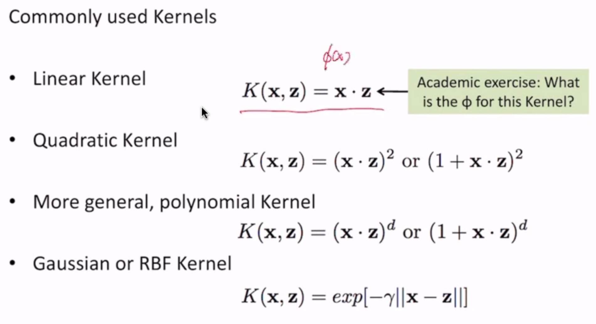
(\(\phi\) for the linear kernel = \(\phi(x) = x\))

Perceptron

we can also apply kernels to perceptron!

Naively, we can just replace \(\mathbf{x}\) with \(\phi(x)\) in the algorithm - but that requires knowledge of \(\phi\)

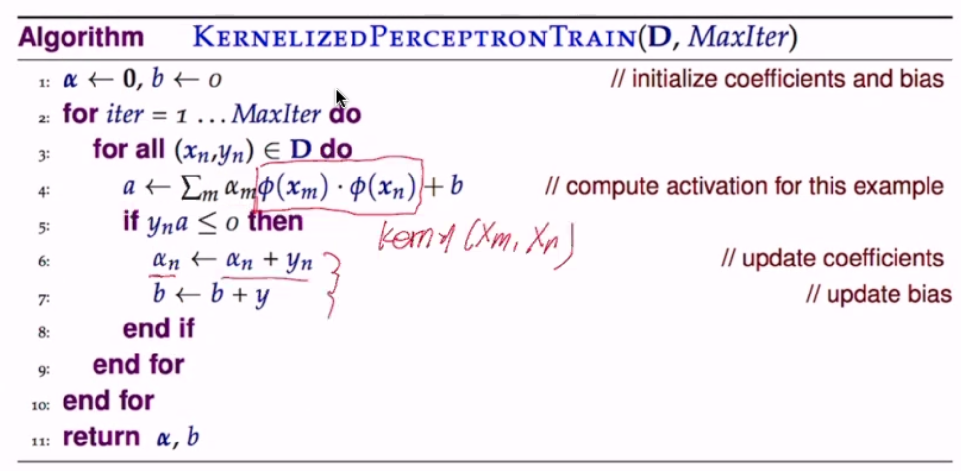
Prediction

since \(w = \sum_m \alpha_m \phi(x_m)\), prediction on \(x_n\) is easy:

\[\hat{y_n} = sign(\sum_m \alpha_m \phi(x_m) \cdot \phi(x_n) + b)\]