Perceptron
Perceptron is a linear, online classification model
Given a training set of pairs, it learns a linear decision boundary hyperplane - we assume labels are binary for now
It’s inspired by neurons: activation is a function of its inputs and weights. For example, the weighted sum activation:
Then, prediction can be something like a > 0 ? 1 : -1.
Additionally, we can add a bias term to account for a non-zero intercept:
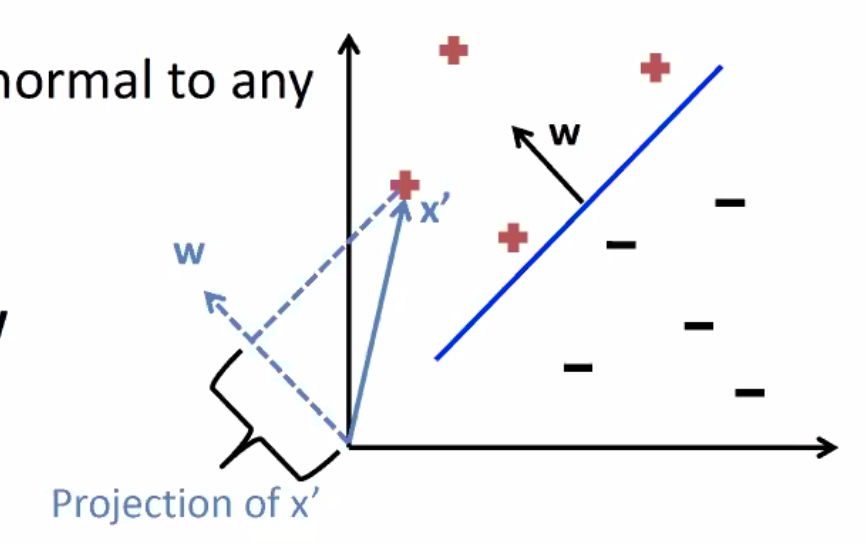
Linear Boundary
- a
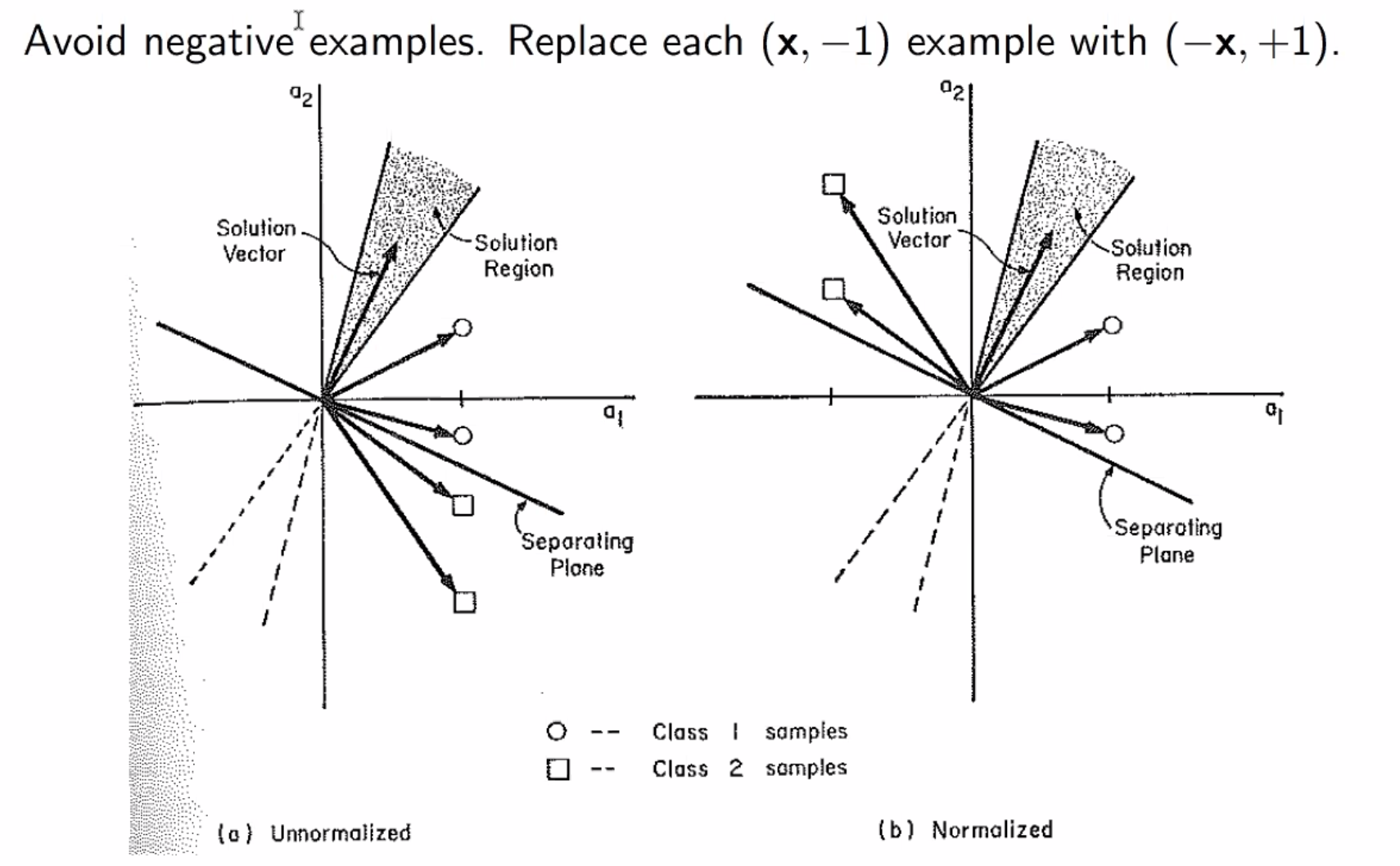
D-1dimensional hyperplane separates aDdimensional space into two half-spaces: positive and negative - this linear boundary has the form \(\mathbf{w} \cdot \mathbf{x} = 0\)
- defined by w: the unit vector (often normalized) normal to any vector on the hyperplane
- \(\text{proj}_w x\) is how far away x is from the decision boundary
- when w is normalized to a unit vector, \(\mathbf{w} \cdot \mathbf{x} = \text{proj}_w x\).
With Bias
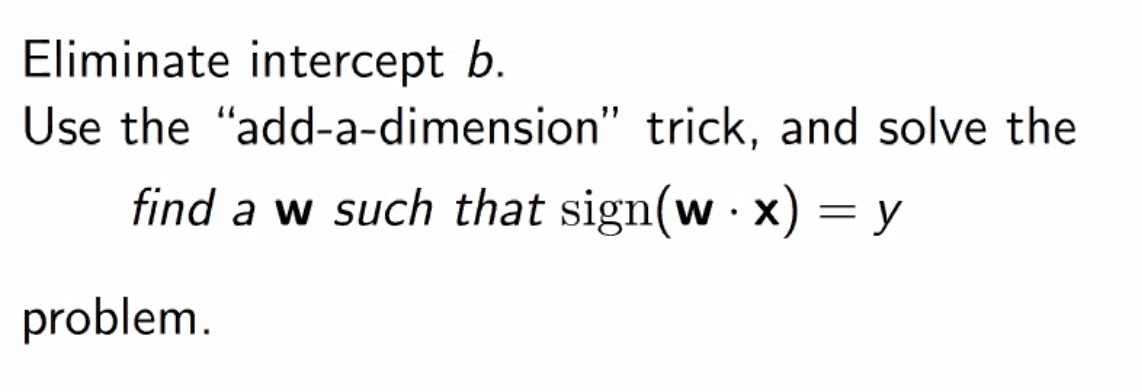
- When a bias is added, the linear boundary becomes \(\mathbf{w} \cdot \mathbf{x} + b = 0\)
- this can be converted to the more general form \(\mathbf{w} \cdot \mathbf{x} = 0\) by adding b to w and an always-1 feature to x
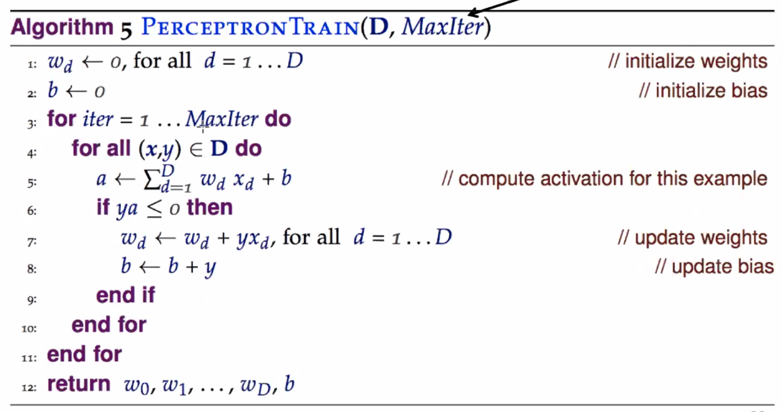
Training
This is an error-driven model:
- initialize model to some weights and biases
- for each instance in training set:
- use current w and b to predict a label \(\hat{y}\)
- if \(\hat{y} = y\) do nothing
- otherwise update w and b to do better
- goto 2
Update in a little simpler notation:
So what does it do? Let’s look at the new activation after an update where a positive was incorrectly predicted as a negative label:
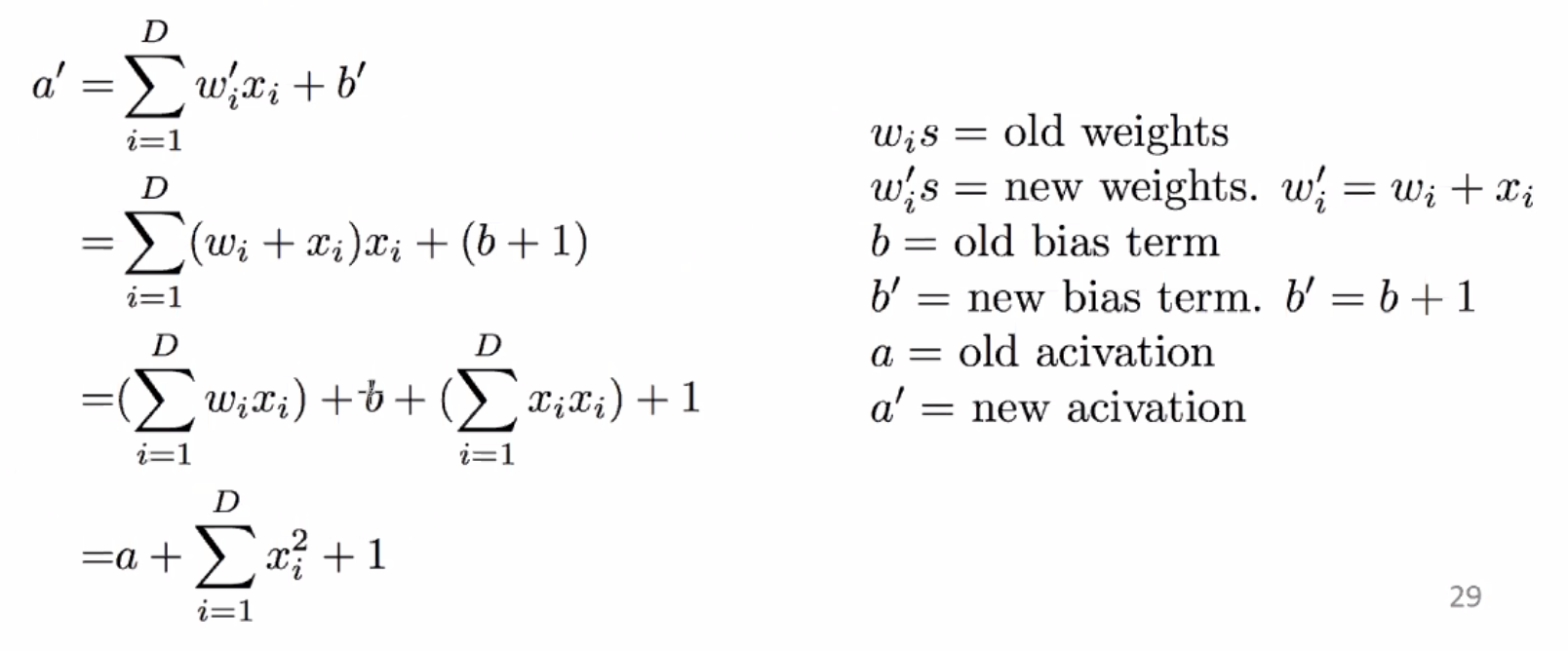
So for the given example, the activation is improved by a factor of positive \(\sum_{i=1}^D x_i^2 + 1\), bringing the prediction closer to correctiveness for that one sample.
We can also control the learning rate easily using a term \(\eta\):
Caveats
- the order of the training instances is important!
- e.g. all positives followed by all negatives is bad
- recommended to permute the training data after each iteration
Example
x1 x2 y  wx  w (after update, if any)
-------------------------------------
             <0, 0>
 1  3  +   0 <1, 3>
 2  3  -  11 <-1, 0>
-3  1  +   3 <-1, 0>
 1 -1  -  -1 <-1, 0>
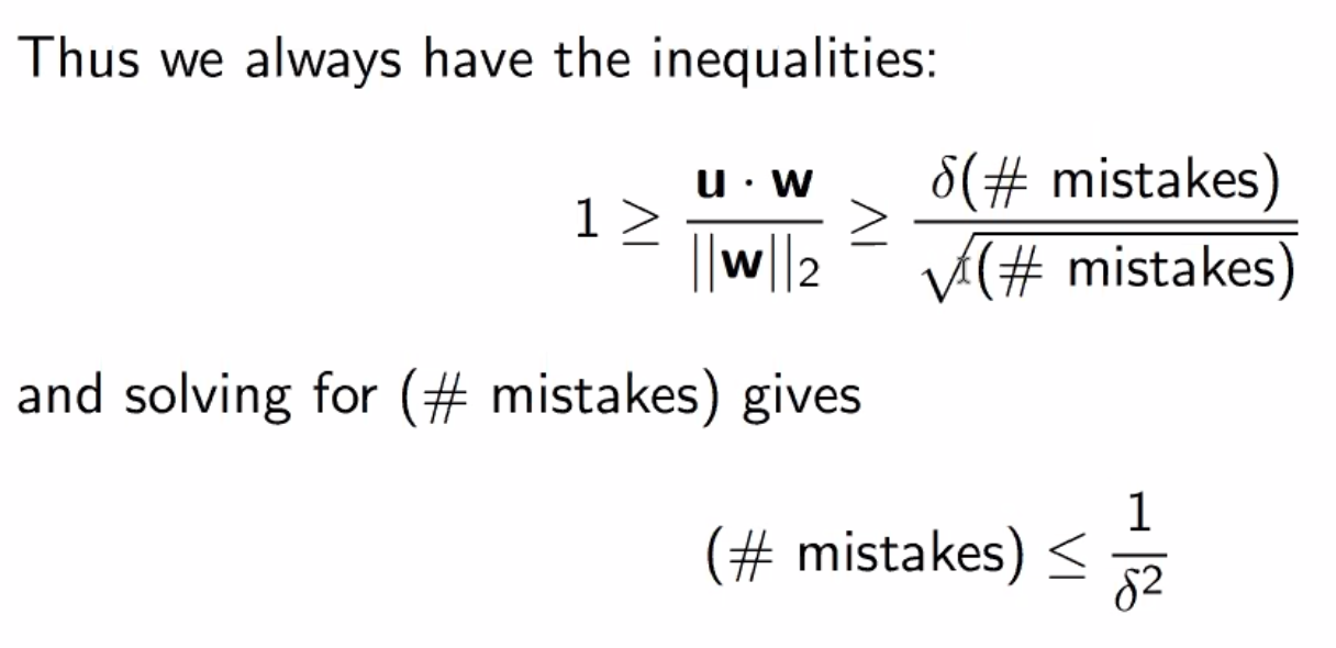
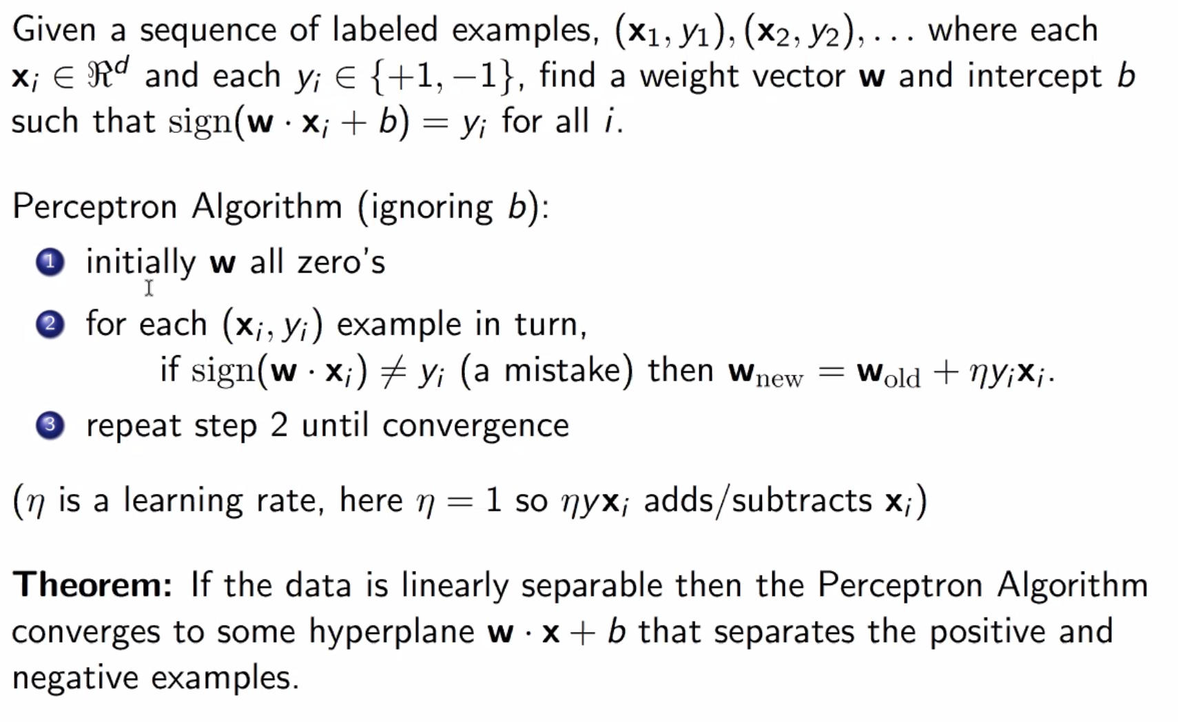
Convergence
We can define convergence as when going through the training data once, no updates are made
If the training data is linearly separable, perceptron will converge - if not, it will never converge.
How long perceptron takes to converge is based on how easy the dataset is - roughly, how separated from each other the two classes are (i.e. the higher the margin is, the easier the dataset is, where margin is the distance from the hyperplane to a datapoint)
Proof
Overview
Steps
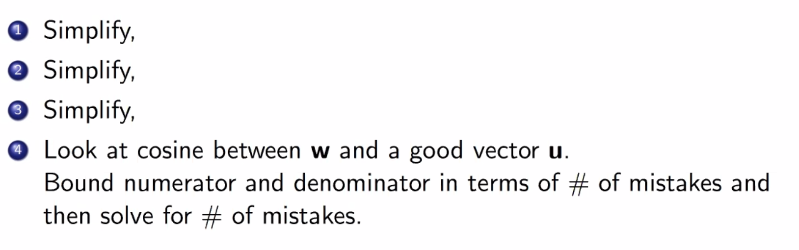
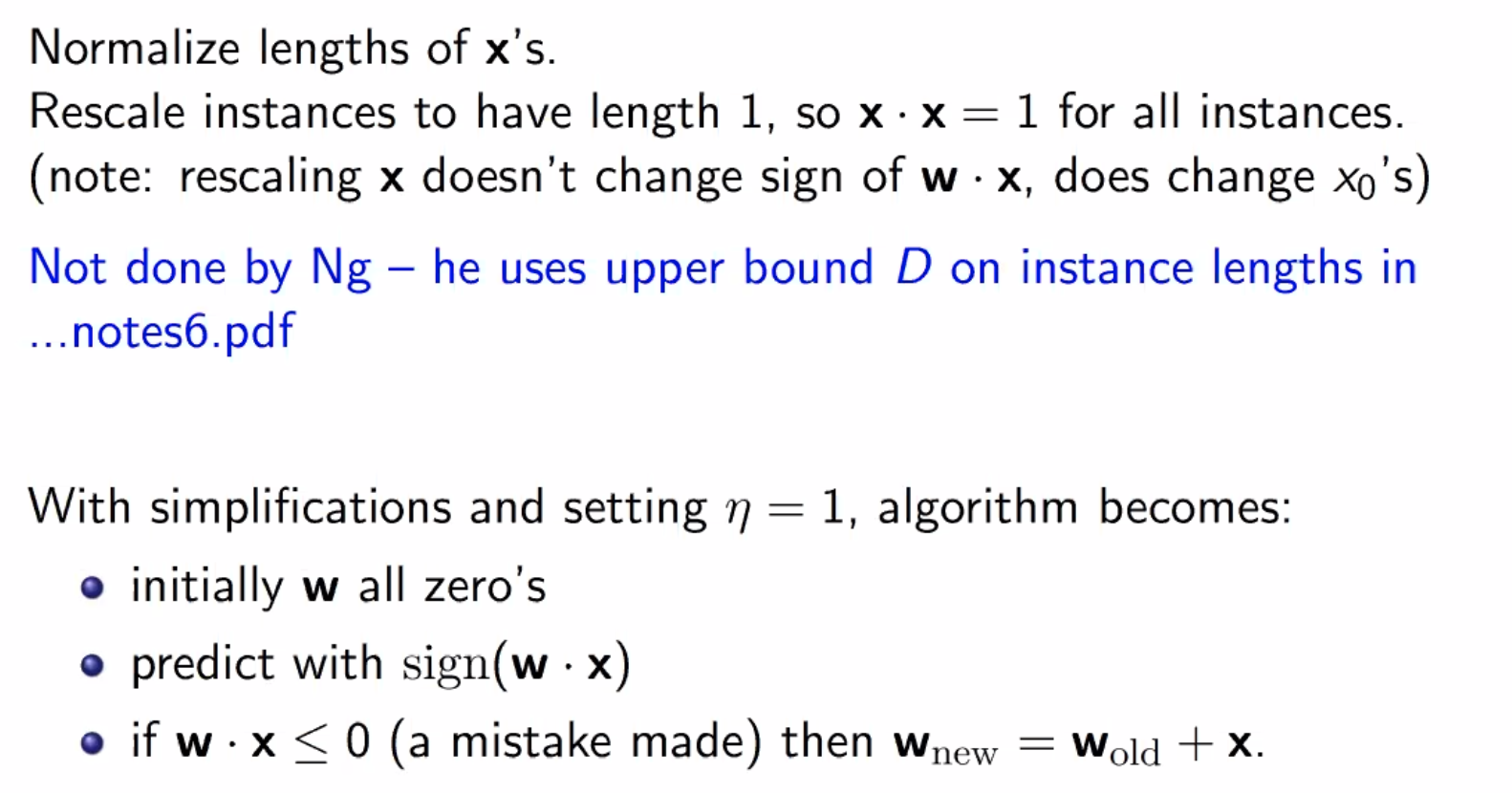
Simplification 1
Simplification 2
Simplification 3
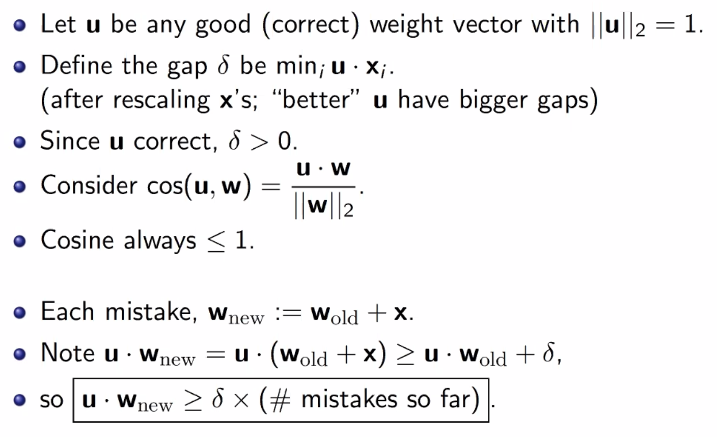
Analysis Setup
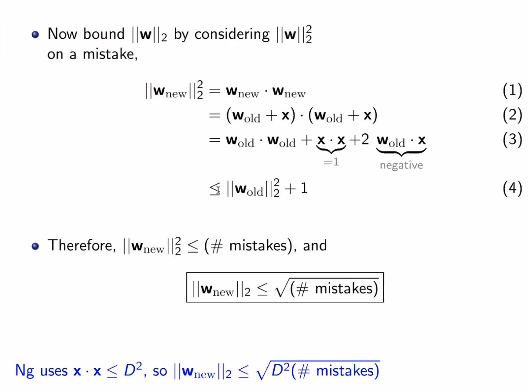
Finishing Up